00:00Hello everyone, in this video we are going to talk about capital allocation across risky and risk-free portfolios
00:11Asset allocation is a very important part of portfolio construction and refers to the choice among broad asset classes
00:18When I say that, I mean that in this framework, we are not referring to specific securities within each asset class, rather our focus is on broad asset class
00:32Before we move on, we also need to ask one more question, and that is, how do we control for risk? The simplest way is to play around with the proportions of the portfolio invested in the risk-free asset and the risky asset
00:50Let us say that Y is the proportion that we allocate to the risky portfolio, and we have given the risky portfolio a name, P, which also means that 1 minus Y is the proportion that is allocated to the risk-free asset, and we have given the risk-free asset also a name, F
01:14If we want to compute the return on the complete portfolio, let us write it as RC, where R stands for the return, and C stands for complete, we can write this as the proportion that we allocate to the risky portfolio, that is Y, multiplied by the return that we obtain from the risky portfolio, let us call that RP, we add to that the return that we derive from The risk-free asset, which is going to be the proportion that is allocated to the risk-free asset, 1 minus y multiplied by the return on the risk-free asset, let's write it as our F
02:06Let us express this equation now in terms of expected return, so if we introduce the expectations operator, we can say that expected return on the complete portfolio is going to be Y times the expected return on the risky portfolio plus one minus y times the return on the risk-free asset
02:35There is no expectation involved with it because it's a risk-free asset
02:44Let us manipulate this equation a little bit, expected return on the Complete portfolio can be written as Y times the expected return on the portfolio, plus we are opening up these brackets, which will mean our RF x 1 is RF, and RF x minus y is minus y RF
03:14Now, let us collect the Y terms together, so the expected return on the complete portfolio is going to be Y, we are collecting the Y terms together, so we write here expected return on the portfolio minus RF, and plus this RF here
03:48We can rewrite this by rearranging the terms, expected return on the complete portfolio is equal to RF plus y times expected return on the portfolio minus RF, while we are at it, let us also write the risk of the
04:22Complete portfolio, which is given by the standard deviation, or Sigma, of the complete portfolio, you will appreciate that all the risk from this put in this portfolio is going to arise from the risky asset, because the risk-free asset, by definition, has no risk, which means that the risk of the complete portfolio is going to be equal to whatever we invest in the risky portfolio multiplied by the standard deviation of the risky portfolio
04:52Let us also write the variance of the risky portfolio, so we are squaring everything up, Y squared times the variance of P
05:16From this part here, we can write the definition of lye, which is going to be Sigma C over Sigma P
05:25Let us keep this in mind, we are going to use this later
05:36Let us now rewrite expected return on our complete portfolio one more time
05:50We have this RF, plus we have a Y here, which we have defined as this, so let us write that, and then inside the bracket, we have this term here
06:24From here, we can identify this slope of this line, which is going to be equal to expected return on the portfolio minus the risk-free rate
06:37We can call this the excess return on the portfolio divided by the standard deviation of the portfolio
06:44You may or may not remember that this ratio is also known as the Sharpe ratio, we also know that risk-averse investors penalize the expected rate of return to account for the risk involved, which means if the risk increases, the penalty should increase as well
07:12But there is a problem, what is going to happen when the return increases with risk? In such a case, the best portfolio is not obvious
07:24What do the investors do then? They assign utility scores to various investments
07:35Let us draw down a particular investor utility function, let us call you as the utility
07:42It is going to be equal to the expected return minus one-half, which we use as a scaling factor, and it is arbitrary
07:57Multiplied by A, which we are going to use as the coefficient of risk aversion
08:06This means the more averse you are to risk, the larger will be the value of A, and this multiplied with the variance, which accounts for the risk
08:24The issue now becomes how to maximize investors' utility by choosing optimum weights for risky and risk-free assets, that is, how much to invest in risky and risk-free asset respectively
08:39Through some calculus, we can maximize the investor utility function with respect to Y, which is the weight on the risky portfolio or the risky asset
08:49Once we know why, the weight on the risk-free asset is simply 1
08:55Minus y, so let us write down our problem
09:00Our problem is to maximize the investor's utility with respect to y, and let us write down the X, let us write down the utility function here one more time
09:14Unit utility increases with expected return and declines or penalized because of risk
09:35Now, let us substitute in you, let us rewrite the utility function again by substituting the definition of expected return on the complete portfolio, which we saw before
09:47This is that definition here, let us copy this and write it here, our F plus y times expected return on the risky portfolio minus the risk-free rate, and after that
10:19We write the penalty one-half times a, and we have to write down the variance now, which we noted before, this was the variance, so let us use this now to complete our utility function, Y squared times Sigma squared P
11:02To maximize the investor utility, we need to take the partial derivative of the utility function with respect to Y and set it equal to zero, and then solve the equation for Y
11:07Let us do that
11:13From this, we get nothing from this term
11:19If we are taking the partial derivative with respect to Y, we get expected return on the portfolio, minus the risk-free rate, now let us look at this term with respect to Y from this
11:42thing here, we are going to get a 2y, so let us write 1 over 2 x - a Y and the variance of the portfolio
11:54This 2 is going to cancel out with this 2, so what are we left with? We have expected return on the portfolio - the risk-free rate - a Y and the variance of the portfolio
12:23Let us set it equal to 0
12:27Once we set it equal to 0, we can take this term to the other side, so this is going to become expected return on the portfolio - the risk-free rate, which is basically our excess return, is going to be equal to a times y times variance of the portfolio
12:49We can very easily find out the value of y from here, we are going to take this guy to the Other side where it's going to get divided, this guy is also going to move over to the other side
13:08Therefore, Y is going to be equal to the excess return divided by A times variance of the portfolio
13:24Let us call it Y star, because this is our optimum weight, this is our optimal weight in the risky portfolio P
13:43This also means that the weight on the risk-free asset is going to be 1 minus Y star
13:53If we do a graphical analysis according to these weights, what we are going to get is known as the capital allocation line
14:08Let us also briefly mention the capital market line before we close this video, we obtain the capital market
14:20Line when, rather than following an active strategy for asset selection, we go for a passively held risky asset like the market index
14:33The market index is a well-diversified portfolio of common stocks, therefore the capital market line is nothing but the capital allocation line, which is formed from a risk-free asset, let us say T-bills, and a broad market index, let's say S&P 500, and we can also call it the market portfolio
15:01The question is, what would be the optimum weight for the risky asset in this case? In this case, the risky asset is the market portfolio, and following the procedure that we just Followed here, this one here, the maximization procedure, we can find the optimum weight in the market portfolio
15:23The only difference is going to be that rather than writing this P here, let me highlight that for you, rather than writing this P here and this P here, we are going to write an M to signify the market
15:37So we can write, in case of us of the CML or the capital market line, the optimum weight or the proportion, the optimum proportion to invest in the market portfolio is going to be the expected return on the market minus the risk-free rate divided by the risk aversion coefficient times the variance of the
16:12Market, this is all I wanted to cover in this video, see you later.