Scal3R: Learning Efficient Multi-Relative Pose Query for Scalable Online 3D Reconstruction

0. Abstract

arXiv:2609.04201 · Chin-Yang Lin, Yang-Che Sun, Cheng Sun, Fu-En Yang, Min-Hung Chen, Yen-Yu Lin, Wei-Chen Chiu, Yu-Lun Liu


Core	Reformulates online 3D reconstruction as multi-reference relative pose querying.
Gap	Global pose regression causes catastrophic drift and geometric collapse on long sequences.
Approach	Injects learnable tokens into a frozen backbone via asymmetric attention + online PGO.
Result	Reduces average ATE by over 60% on KITTI compared to the online baseline.

The Problem with Online 3D Reconstruction — Online 3D reconstruction models struggle with long videos due to accumulated drift and geometric collapse. [8]

Problem with existing models [8]
1. Existing online 3D reconstruction models perform poorly on long videos. [8]
2. This is because they regress poses relative to a fixed first-frame anchor. [8]
3. This forces extrapolation far beyond the training distribution. [9]
4. Small drifts accumulate and amplify into significant geometric collapse. [9]
Observation motivating Scal3R [10]
1. Per-frame depth remains stable even when global pose fails. [10]
2. The backbone's local geometry stays intact, but the global pose head breaks down. [10]
3. This decoupling motivates Scal3R. [11]
Scal3R's approach [11]
1. Scal3R reformulates online reconstruction as multi-reference relative pose querying. [11]
2. It uses lightweight learnable tokens, which are about ~1% of the parameters. [12]
3. These tokens are injected into a completely frozen backbone via asymmetric attention. [12]
4. This setup queries poses relative to multiple past keyframes. [13]
Drift suppression and performance [13]
1. An online pose-graph optimization (PGO) system with loop closure suppresses long-range drift. [13]
2. Scal3R converges in 8 hours on a single GPU. [14]
3. It reduces the average Absolute Trajectory Error (ATE) by over 60% on KITTI compared to the online baseline. [14]
4. It achieves state-of-the-art performance across Virtual KITTI, Sintel, TUM-Dynamic, ScanNet, and 7-Scenes. [15]

1. Introduction

Feed-forward models like CUT3R and STream3R enable real-time 3D reconstruction. [16] They decode per-frame geometry into a unified global coordinate system by directly regressing poses relative to the first frame. [17] This global anchor paradigm works well for short sequences but faces severe stability and scalability bottlenecks in long-range environments. [18]

Fundamental issues with global pose regression [19]
1. Limited scene scales in training data [19]
  1. Existing 3D datasets cover limited scene scales. [19]
  2. Models trained on short sequences must extrapolate to global coordinates far outside their training distribution. [19]
  3. When deployed on real-world trajectories spanning hundreds of meters, minor feature drift is amplified into geometric collapse. [20]
2. Highly variable camera motions [21]
  1. Real-world camera motions are highly variable. [21]
  2. For unbounded video streams, the global coordinate system inevitably encounters out-of-distribution trajectories. [21]
  3. This makes feed-forward global pose regression theoretically unable to scale. [22]
Localized failure observation [23]
1. Failure is highly localized. [23]
2. Global pose errors diverge catastrophically, but per-frame depth remains consistently stable. [23]
3. This indicates that the backbone's local geometric representations are intact. [24]
4. The failure is isolated to the global pose regression head. [24]
Scal3R's shift in approach [24]
1. Scal3R shifts from global pose regression to local relative querying. [24]
2. It exploits the well-learned local geometry to estimate stable relative transformations. [25]
3. This is done via a visual query mechanism conditioned on reference viewpoints. [25]
4. The backbone remains entirely frozen. [26]

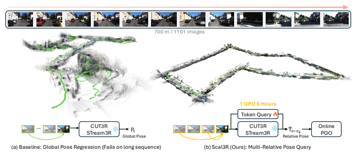Scal3R enables scalable online 3D reconstruction on long video streams.

Figure 1: Scal3R enables scalable online 3D reconstruction on long video streams. [4] (a) Baseline: Global Pose Regression (Fails on long sequence). (b) Scal3R (Ours): Multi-Relative Pose Query. [3]

Scal3R framework details [27]
1. Scal3R is an efficient framework for scalable online 3D reconstruction. [27]
2. A small set of learnable tokens is injected into the frozen backbone via asymmetric attention. [27]
3. Pose tokens attend to image features as queries. [28]
4. Image tokens compute self-attention exclusively among themselves, preserving the frozen representation space. [28]
5. Each pose token predicts the relative transformation between the current frame and a historical reference. [29]
6. This constrains localization to the local viewpoint domain where the model is most reliable. [29]
7. To maintain global consistency, Scal3R incorporates multi-reference relative querying and online pose-graph optimization (PGO). [30]
8. Relative poses are queried against multiple dynamically selected reference frames simultaneously. [31]
9. These are aggregated via PGO into a drift-free trajectory. [31]
10. A loop closure mechanism integrates naturally into the multi-reference pipeline. [32]

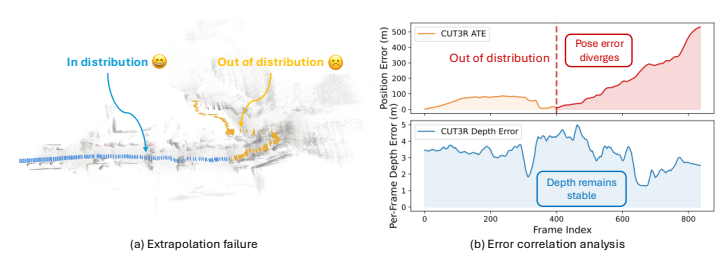Global pose regression fails under out-of-distribution sequences, while local geometry remains reliable.

Figure 2: Global pose regression fails under out-of-distribution sequences, while local geometry remains reliable. [37] (a) Extrapolation failure. (b) Error correlation analysis. [33]

Summary of contributions [42]
1. Identified that global extrapolation instability and limited training data coverage cause long-sequence collapse in 3D reconstruction. [42]
2. Showed that local geometric representations remain reliable throughout this failure. [43]
3. Proposed Scal3R, which introduces multi-reference relative pose querying via visual prompt tuning on a frozen backbone. [44]
4. Asymmetric attention injection ensures that pose learning does not degrade point cloud quality. [44]
5. Integrating multi-reference querying with online PGO, Scal3R achieves low drift on kilometer-scale sequences. [45]
6. It converges in about 8 hours on a single GPU using only 4-view training samples. [46]

2. Related Work

Multi-view 3D Reconstruction [47]
1. Early reconstruction relied on offline Structure-from-Motion and Multi-View Stereo pipelines. [47]
2. Optimization-based approaches jointly refine camera poses with scene representation but are per-scene and offline. [48]
3. Feed-forward methods dramatically improved efficiency by predicting geometry in a single forward pass. [48]
4. Recent transformer-based models scale to large unordered collections via joint pose-and-geometry prediction and efficient aggregation strategies. [49]
5. A complementary trend adapts frozen 3D foundation models for downstream tasks without backbone retraining. [51]
6. Scal3R follows this paradigm but uniquely targets scalable pose estimation on unbounded video streams where batch-processing systems cannot operate. [52]
Online 3D Reconstruction [53]
1. Online methods shift from batch processing to incremental inference, processing video frame by frame. [53]
2. This is achieved through recurrent TSDF fusion, differentiable bundle adjustment, and progressive radiance-field optimization. [54]
3. CUT3R and STream3R bring this to 3D foundation models via persistent state updates and causal Transformers. [54]
4. This spawned a broad family of streaming systems and SLAM integrations. [55]
5. However, all share a critical flaw: poses are regressed relative to the first frame, anchoring the trajectory to a single global reference. [56]
6. This strategy becomes increasingly fragile as sequences grow, amplifying small feature drifts into catastrophic geometric collapse. [56]
Long-sequence Streaming 3D Reconstruction [58]
1. Suppressing drift over kilometer-scale sequences remains an open challenge. [58]
2. Approaches include test-time gradient updates, training-free memory management, long-range token pools, explicit spatial memory, stage-decoupled streaming, and offline global optimization. [58]
3. Each approach trades off online capability against global consistency. [60]
4. Earlier per-scene methods handle long casual videos by incrementally estimating poses with learned 3D priors or progressively allocating local radiance fields rather than a single global representation. [60]
5. This was an early departure from single-anchor formulations. [62]
6. A unifying insight from visual odometry literature is that relative formulations generalize better than absolute ones. [62]
7. This insight guides Scal3R. [63]
8. Scal3R reformulates the problem as multi-reference relative pose querying on a frozen backbone, eliminating the root extrapolation failure with only ~1% additional parameters. [63]
Efficient Prompt Tuning [65]
1. Parameter-efficient adaptation shows that frozen pre-trained models need very little change to transfer well. [65]
2. Adapters, prefix tokens, soft prompts, low-rank perturbations, and parallel adapter modules all match or exceed full fine-tuning at under 2% of parameters. [65]
3. This finding is confirmed broadly across vision transformers. [66]
4. This paradigm has reached 3D vision, where geometry-aware prompts and low-rank adapters on frozen 3D transformers and reconstruction backbones consistently match full fine-tuning. [67]
5. Attention-level token gating on a frozen large reconstruction model enables mesh editing without backbone retraining. [68]
6. Human3R first demonstrated prompt tuning on a frozen CUT3R for joint human-scene reconstruction. [69]
7. Scal3R is the first to apply this paradigm to relative pose estimation. [70]
8. It recasts it as a multi-reference prompt query task via asymmetric attention injection. [70]
9. This preserves the backbone's pointmap quality while gaining globally consistent motion representations. [71]

3. Method

3.1. Overview [80]

Scal3R addresses online 3D reconstruction by reformulating global pose regression as a multi-reference relative pose query problem. [81]

Problem reformulation [81]
1. Given a streaming sequence of images, Scal3R queries relative poses with respect to a set of maintained reference frames. [81]
2. It does not directly regress absolute camera poses in a unified world coordinate system. [82]
3. This reformulation fundamentally eliminates the long-horizon extrapolation instability that plagues existing global-regression approaches. [83]
Architectural components [84]
1. Scal3R builds upon frozen pretrained online 3D reconstruction backbones (e.g., CUT3R or STream3R). [84]
2. It preserves their rich spatiotemporal geometric priors. [85]
3. A lightweight set of learnable tokens is injected into the frozen decoder via an asymmetric attention mechanism. [85]
4. This enables relative pose decoding without modifying the pretrained weights. [86]
5. At the backend, an online Pose-graph Optimization (PGO) module aggregates the predicted pairwise relative constraints into a globally consistent trajectory. [86]
6. Figure 3 shows an overview of the full pipeline. [87]

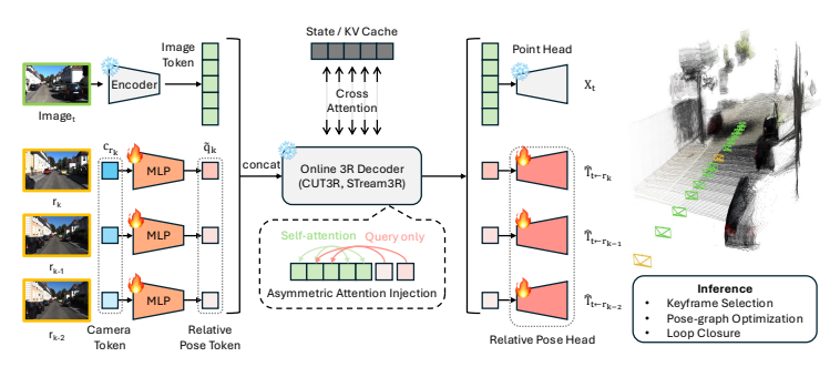Overview of the Scal3R framework.

Figure 3: Overview of the Scal3R framework. [75]

3.2. Preliminaries: Online 3D Reconstruction Backbones [88]

Scal3R builds upon two representative backbone paradigms. [88]

Persistent state model (CUT3R) [89]
1. At each timestep t, the frozen online 3D reconstruction backbone processes the current frame It together with a persistent hidden state St-1. [89]
2. St-1 encodes the scene history. [90]
3. This produces an updated state St and local geometry prediction Gt. [90]
Causal Transformer model (STream3R) [90]
1. At each timestep t, the frozen online 3D reconstruction backbone processes the current frame It via causal attention over a sliding feature window {Ft-k, ..., Ft}. [90]
2. This performs cross-temporal geometric alignment in feature space. [91]
3. This produces local geometry prediction Gt. [92]
Common decoding structure and its limitations [92]
1. Both paradigms share a common decoding structure. [92]
2. At each frame, the decoder maintains image feature tokens Ft ∈ R H×W×C and a dedicated camera token ct ∈ R D. [93]
3. Pointmaps are decoded from Ft for local geometry. [93]
4. The global camera pose Pt ∈ SE(3) relative to the first frame is regressed from ct. [94]
5. Although effective for short sequences, global-reference regression degrades over long sequences. [94]
6. As the sequence grows, the model must align each new frame to an increasingly distant first-frame coordinate system. [95]
7. This causes small feature drifts to be amplified into severe geometric collapse at the decoding stage. [95]
Scal3R's modification [96]
1. Scal3R retains the rich representations Ft and ct learned by these backbones. [96]
2. It discards their unstable global pose regression heads. [97]
3. Instead, it leverages historical camera tokens {crk} stored in the pose token buffer as geometric conditioning signals to enable scalable relative pose queries. [97]

3.3. Multi-Reference Relative Pose Tuning [98]

Scal3R's core contribution is a parameter-efficient prompt tuning mechanism. [98] This enables robust multi-reference relative pose prediction on a completely frozen backbone. [98]

Parameter efficiency [99]
1. The total number of newly introduced parameters accounts for ~1% of the backbone's total parameter count. [99]
Multi-reference query mechanism [100]
1. To query multiple reference viewpoints simultaneously, Scal3R maintains a pose token buffer. [100]
2. This buffer stores the camera tokens of selected past keyframes. [101]
3. A shared base query token q ∈ R D is learned. [101]
4. This token serves as a query template, directing the decoder to extract the geometric relationship between the current frame and a given reference frame. [102]
5. For each reference slot k, the corresponding reference frame features retrieved from the buffer are projected into feature space via a lightweight MLP. [102]
6. These are fused with the base token by additive injection: [103] $\tilde{q}_{k} = q + MLP (c_{r_{k}})$ where crk is the camera token of the k-th reference frame. [104]
7. This dynamic assembly allows the system to flexibly scale the number of active queries K based on available references. [104]
8. This ensures robustness during sequence initialization or buffer resets. [105]
9. The number of reference frames can be freely extended at inference time without retraining because each token queries independently. [106]

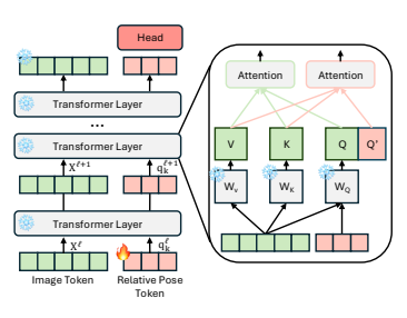Asymmetric Attention Injection.

Figure 4: Asymmetric Attention Injection. [113]

Asymmetric Attention Injection [117]
1. Naively inserting new tokens into the decoder's self-attention would perturb the attention distribution of image tokens. [117]
2. This would degrade pointmap reconstruction quality. [118]
3. Scal3R proposes asymmetric attention injection (Figure 4). [118]
4. Pose query tokens {q˜k} participate in decoder attention exclusively as queries. [118]
5. They attend to all image tokens to extract geometric features. [119]
6. Image tokens compute their Keys and Values without attending to the pose query tokens. [119]
7. For a decoder layer with image tokens X: [120] $\tilde{q}_{k}^{ℓ + 1} = Attention (Q = \tilde{q}_{k}^{ℓ}, K = X^{ℓ}, V = X^{ℓ})$ $X^{ℓ + 1} = SelfAttention (X^{ℓ})$
8. This one-directional information flow guarantees that the image feature representation space remains identical to that of the original frozen model. [121]
9. This fully preserves pointmap reconstruction fidelity. [122]
10. No attention mask is needed, as pose tokens never enter the image K/V sequence. [122]
Relative Pose Decoding and Loss [123]
1. After multi-layer feature exchange, each pose query token q˜k encapsulates the relative geometric constraint between the current frame t and its corresponding reference frame rk. [123]
2. A lightweight MLP head decodes these tokens into relative poses. [124]
3. The 6D rotation representation is adopted to ensure continuity in the rotation space. [124]
4. The relative transformation is output: [125] $\hat{T}_{t \leftarrow r_{k}} = Head (\tilde{q}_{k}) \in S E (3)$
5. The training loss supervises rotation R and translation t separately. [126]
6. Rk pred and t k pred denote the rotation matrix and translation vector decomposed from Tˆ t←rk. [126]
7. Rk gt and t k gt are the corresponding ground-truth components. [127]
8. To handle monocular scale ambiguity, translation vectors are scale-aligned before loss computation. [127]
9. The total loss aggregates over all K reference links: [128] $L = k = 1 \sum K (λ_{R} R_{p r e d}^{k} - R_{g t}^{k}_{F} + λ_{t} t_{p r e d}^{k} - t_{g t}^{k}_{2})$ where λR and λt are loss weighting hyperparameters. [129]

3.4. Online Pose-graph Optimization [130]

Naively chaining multi-reference relative pose predictions accumulates drift over long sequences. [130] Scal3R integrates an online pose-graph optimization (PGO) framework. [131] This uses predicted relative poses as between-factors and performs incremental trajectory correction as new frames arrive. [131]

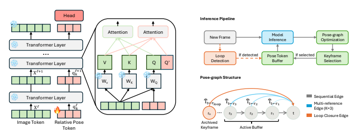Inference pipeline and pose graph structure.

Figure 5: Inference pipeline and pose graph structure. [113]

Keyframe Selection [133]
1. Including every frame in the pose graph introduces numerical redundancy and unnecessary computation. [133]
2. An online 3D overlap-based keyframe selection strategy is adopted. [134]
3. A KD-tree spatial index maintains the reconstructed 3D point cloud. [134]
4. The visible point set for each frame is determined by projecting predicted 3D points onto a unit sphere. [135]
5. Angular overlap with past keyframes is computed to avoid interference from geometrically non-adjacent regions. [136]
6. For each incoming frame t, predicted 3D points are transformed to world coordinates via the current pose estimate. [137]
7. If the depth-normalized overlap score falls below a threshold τoverlap and the median depth confidence exceeds τconf, the frame is designated as a keyframe. [137]
8. This indicates novel geometry with reliable prediction quality. [138]
9. Only keyframes update the frozen decoder's KV cache and enter the pose token buffer. [138]
10. Non-keyframe KV states are discarded by restoring the pre-forward snapshot, keeping the streaming decoder state clean. [139]
11. The first Ninit frames are unconditionally treated as keyframes to initialize the system. [139]
Pose-graph Optimization [140]
1. The trajectory is modeled as a factor graph where each camera pose Tt ∈ SE(3) is a variable node. [140]
2. Multi-reference relative poses form between-factors connecting the current frame to its Kt references: [141] $E_{between} = t \sum k = 1 \sum K_{t} ρ (lo g (T_{r_{k}}^{- 1} T_{t} \cdot \hat{T}_{t \leftarrow r_{k}})_{Σ_{t, k}}^{2})$
3. Tˆ t←rk is the predicted relative pose. [142]
4. Σt,k is a diagonal noise covariance. [142]
5. ρ(·) is the Huber robust kernel to downweight outlier constraints. [143]
6. To account for higher uncertainty in predictions between temporally distant frame pairs, a gap-dependent noise model is adopted. [143]
7. The standard deviation scales as σ = σbase · ∆0.5 with frame gap ∆. [144]
8. iSAM2 is employed for incremental optimization. [144]
9. Upon each new frame arrival, the factor graph is updated and efficiently re-optimized via the Bayes tree structure. [145]
10. Optimized poses are written back to the buffer so that subsequent frames use corrected references. [146]
11. For long sequences, the frozen decoder's streaming state is reset every Nreset frames to prevent memory overflow and feature degradation. [147]
12. To maintain pose graph connectivity across resets, the last frame of each segment is re-fed as the first frame of the next segment. [147]
13. A tight identity constraint is imposed between the two corresponding nodes in the factor graph. [148]
Loop Closure [149]
1. Despite PGO continuously correcting local drift, long-term trajectory consistency requires explicitly detecting and closing loops. [149]
2. This happens when the camera revisits previously observed regions. [149]
3. A key advantage of the multi-reference design is that loop closure integrates naturally into the existing inference pipeline. [150]
4. When a loop candidate is detected between the current frame t and a past keyframe rloop, the archived camera token of rloop is re-injected into the pose token buffer as an additional reference slot. [150]
5. The frozen model then predicts a long-range relative pose constraint Tˆ t←rloop without any architectural modification. [151]
6. This is added to the pose graph as a high-confidence edge with a tight Gaussian noise model. [151]
7. For loop detection, a pretrained DINOv2 backbone with a SALAD aggregation layer is employed. [151]
8. This produces discriminative scene-level descriptors, indexed online via FAISS over keyframes only. [152]
9. Candidates are filtered by cosine similarity threshold τsim, minimum temporal gap τgap, and non-maximum suppression within a window wnms to suppress redundant detections. [153]

4. Experiments

4.1. Implementation Details [155]

Model Configurations [155]
1. Scal3R builds upon two representative online 3D reconstruction backbones: CUT3R and STream3R. [155]
2. CUT3R centers on persistent state updates. [156]
3. STream3R is based on causal Transformers. [156]
4. Experiments employ their 24-layer Transformer backbones (comprising a DINOv2 encoder and a Transformer decoder). [157]
5. These are kept entirely frozen to leverage their strong spatiotemporal geometric priors. [157]
6. For each incoming frame, a set of lightweight, learnable relative pose query tokens is introduced. [158]
7. These tokens account for only approximately 1% of the total model parameters. [159]
8. These tokens are injected into the decoder layers via asymmetric attention injection to extract geometric constraints of the current frame relative to the reference frames in the pose token buffer. [159]
9. A pose decoding head then maps these features into SE(3) space, predicting the 6D rotation and translation vectors. [161]
Training [171]
1. The model is fine-tuned on the TartanAir dataset, which provides diverse scenarios and precise trajectory ground truth. [171]
2. A Random Interval Sampling strategy is adopted during training to ensure robustness to varying motion velocities and baseline lengths. [172]
3. For each training sample, 4 views are selected from a sequence. [173]
4. One view serves as the current frame It, and the remaining three as reference frames (K = 3). [173]
5. Temporal intervals between frames are randomly perturbed. [174]
6. This mechanism forces the model to extract stable relative pose representations under varying levels of geometric constraint. [174]
7. Since each pose query token attends independently, the number of reference frames can be freely scaled at inference time without retraining. [175]
8. K = 12 is used during inference. [176]
9. For long outdoor benchmarks (KITTI and vKITTI), the frozen decoder's streaming state is reset every Nreset = 10 frames. [176]
10. All other datasets use no reset. [177]
11. Training is performed with a batch size of 8 for 40 epochs using the AdamW optimizer with a learning rate of 1 × 10−4. [177]
12. The entire fine-tuning converges in approximately 8 hours on a single NVIDIA A100 GPU. [178]
13. This avoids the collapse of geometric priors commonly observed in full-parameter fine-tuning on small-scale datasets. [179]
Baselines [180]
1. Scal3R is compared with offline transformers, streaming models, and SLAM-style systems. [180]
2. Offline transformers include VGGT, π3, Fast3R, and DA3. [180]
3. Streaming baselines include CUT3R, MUSt3R, TTT3R, STream3R, WinT3R, StreamVGGT, and Point3R. [181]
4. MASt3R-SLAM is included as an incremental SLAM counterpart. [181]
5. All methods operate in an intrinsic-free setting, taking only RGB input without known camera intrinsics. [181]
6. They are evaluated with official default settings under a unified protocol. [181]

4.2. Quantitative Results [194]

Camera Pose Estimation [194]

Average Trajectory Error (ATE) is evaluated across multiple benchmarks. [194]
Benchmarks include KITTI and Virtual KITTI (vKITTI) for outdoor driving scenarios. [195]
Sintel, TUM-Dynamic, and ScanNet are used for diverse indoor and synthetic environments. [195]
Sim(3) alignment is applied to the ground truth before computing ATE, following CUT3R and STream3R. [196]
Scal3R consistently outperforms both offline and online baselines. [197]

Methods	00	01	02	03	04	05	06	07	08	09	10	Avg.
VGGT [80]	-	-	-	-	-	-	-	-	-	-	-	-
Fast3R [92]	-	723.1	-	166.9	112.2	-	137.4	90.9	-	225.6	211.7	238.3
DA3 [47]	-	-	-	-	12.6	-	-	-	-	-	-	12.6
π 3 [86]	-	-	-	-	2.3	-	-	-	-	-	-	2.3
MASt3R-SLAM [57]	188.5	562.9	282.4	121.7	92.6	-	57.2	77.0	263.6	184.1	179.1	200.9
MUSt3R [5]	-	490.1	-	121.5	58.1	-	100.6	66.8	-	-	-	167.4
CUT3R [82]	191.0	644.1	295.4	150.1	20.1	155.6	132.7	72.8	231.8	206.2	179.6	207.2
Point3R [89]	-	-	-	-	-	-	-	-	-	-	-	-
STream3R [40]	189.0	694.9	302.6	162.7	100.5	159.1	122.7	87.1	264.5	220.9	195.9	227.3
WinT3R [44]	-	698.1	-	144.5	89.4	150.8	135.8	76.0	242.8	200.9	210.3	216.5
StreamVGGT [104]	-	-	-	-	98.8	-	-	-	-	-	-	98.8
TTT3R [11]	178.4	529.1	280.8	98.0	11.4	147.9	132.1	70.2	240.2	191.0	125.2	182.2
Ours (CUT3R)	45.3	165.0	139.9	33.9	9.9	29.4	47.4	6.4	227.0	29.6	33.2	69.7
Ours (STream3R)	57.9	176.4	170.8	10.9	9.3	39.1	18.1	15.2	173.8	73.9	33.9	70.8

Table 1: Camera pose estimation on KITTI (ATE ↓). Scal3R reduces average ATE by over 60% compared to the strongest online competitor TTT3R, with particularly pronounced gains on long-range sequences. [163]

On KITTI (Table 1), Scal3R achieves an average ATE of 69.7. [197]
This reduces error by over 60% compared to the strongest online competitor TTT3R (182.2). [198]
Gains are particularly pronounced on long-range sequences such as Seq. 00 and Seq. 02. [198]

Methods	Scene01	Scene02	Scene06	Scene18	Scene20	Avg.
VGGT [80]	-	0.22	-	-	-	0.22
Fast3R [92]	72.71	23.72	6.05	58.93	159.40	64.16
DA3 [47]	25.22	0.22	0.17	12.53	182.89	44.20
π 3 [86]	4.63	0.33	0.18	3.04	-	2.04
MASt3R-SLAM [57]	75.16	-	7.056	-	-	41.11
MUSt3R [5]	77.23	7.39	0.28	48.53	170.91	60.87
CUT3R [82]	59.76	29.73	0.65	44.89	146.92	56.39
Point3R [89]	75.70	30.44	4.81	62.85	138.24	62.41
STream3R [40]	66.83	25.47	1.52	68.18	223.07	77.01
WinT3R [44]	59.02	28.61	1.10	42.89	203.16	66.96
StreamVGGT [104]	55.09	32.91	0.57	57.18	-	36.44
TTT3R [11]	29.05	12.15	0.54	6.75	77.90	25.28
Ours (CUT3R)	4.50	0.72	0.66	5.56	16.72	5.63
Ours (STream3R)	5.39	3.26	3.21	6.40	21.32	7.92

Table 2: Camera pose estimation on Virtual KITTI (ATE ↓). Scal3R surpasses all streaming methods by a large margin and approaches the accuracy of offline approaches on long-range sequences. [182]

On vKITTI (Table 2), Scal3R (CUT3R) attains an average ATE of 5.63. [199]
This surpasses all streaming methods by a large margin. [199]
It approaches the accuracy of the offline method π3 while remaining fully online. [200]

| Methods | Sintel | TUM | ScanNet | |---|---|---| | MASt3R-SLAM [57] | 0.233 | 0.103 | 0.081 | | MUSt3R [5] | 0.242 | 0.048 | 0.046 | | CUT3R [82] | 0.210 | 0.049 | 0.095 | | Point3R [89] | 0.375 | 0.067 | 0.120 | | STream3R [40] | 0.214 | 0.026 | 0.052 | | WinT3R [44] | 0.225 | 0.074 | 0.062 | | StreamVGGT [104] | 0.394 | 0.057 | 0.120 | | TTT3R [11] | 0.210 | 0.028 | 0.064 | | Ours (CUT3R) | 0.168 | 0.033 | 0.092 | | Ours (STream3R) | 0.171 | 0.018 | 0.049 |

Table 3: Camera pose estimation on Sintel, TUM-Dynamic, and ScanNet (ATE ↓). Scal3R achieves state-of-the-art performance across all three benchmarks. [182]

On Sintel, TUM-Dynamic, and ScanNet (Table 3), Scal3R generalizes robustly to unseen domains. [200]
Scal3R (CUT3R) achieves the best ATE of 0.168 on Sintel. [201]
Scal3R (STream3R) attains state-of-the-art ATE of 0.018 on TUM-Dynamic and 0.049 on ScanNet. [201]
This demonstrates strong performance across both large-scale outdoor and dense indoor environments without sacrificing online processing. [202]

3D Reconstruction [203]

3D reconstruction quality is evaluated on the 7-Scenes dataset using 300-frame sequences. [203]
Metrics reported are Accuracy (Acc.), Completeness (Comp.), and Normal Consistency (NC). [204]
Scal3R variants consistently enhance the geometric consistency of their frozen backbones. [204]

Methods	Acc. ↓ Mean	Acc. ↓ Med.	Comp. ↓ Mean	Comp. ↓ Med.	NC ↑ Mean	NC ↑ Med.
CUT3R [82]	0.130	0.090	0.062	0.023	0.544	0.565
STream3R [40]	0.095	0.040	0.030	0.006	0.560	0.590
Ours (CUT3R)	0.069	0.034	0.035	0.010	0.566	0.601
Ours (STream3R)	0.052	0.012	0.020	0.004	0.579	0.622

Table 4: 3D reconstruction on 7-Scenes (300 frames). Scal3R consistently improves upon both CUT3R and STream3R backbones, achieving the best NC across all sequences. [206]

Ours (STream3R) achieves the best performance across all metrics (Table 4). [205]
It attains an NC mean of 0.579 and median of 0.622. [205]
This surpasses the STream3R backbone by a clear margin. [207]
Competing streaming methods struggle to improve geometric consistency beyond their base backbone. [207]
Scal3R's scale-decoupled formulation yields consistent gains in NC without sacrificing accuracy or completeness. [208]

4.3. Qualitative Results [211]

3D Reconstruction [211]
1. Figures 6 and 7 visualize 3D reconstruction and trajectory estimation on outdoor long-sequence benchmarks. [211]
2. This confirms stable reconstruction and pose prediction across varying spatial extents. [212]
3. For 3D reconstruction (Figure 6), Scal3R is compared against CUT3R and STream3R on Virtual KITTI Scene 01 (332 m) and Scene 02 (113 m). [212]
4. CUT3R produces severely distorted point clouds with substantial geometric drift. [213]
5. STream3R collapses into degenerate reconstructions that deviate considerably from the ground-truth layout. [214]
6. Both Ours (CUT3R) and Ours (STream3R) recover scene geometry that closely matches the ground truth. [214]
7. They show clean structural boundaries and well-preserved spatial extent. [214]

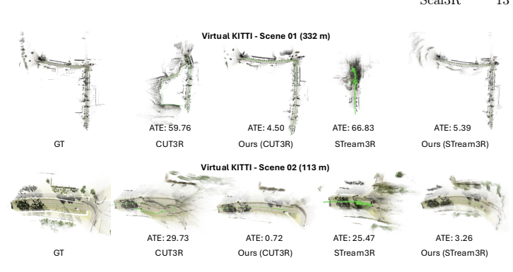Qualitative 3D reconstruction on Virtual KITTI.

Figure 6: Qualitative 3D reconstruction on Virtual KITTI. [220]

Long-sequence Pose Estimation [215]
1. For long-sequence pose estimation (Figure 7), estimated trajectories on KITTI Seq. 00 and Seq. 05 are visualized against CUT3R, WinT3R, and STream3R. [215]
2. All three baselines suffer from catastrophic trajectory collapse. [215]
3. They produce chaotic, self-intersecting paths that bear no resemblance to the ground-truth loop structure. [216]
4. In contrast, Ours (CUT3R) faithfully traces the full loop trajectory. [216]
5. It maintains metric accuracy and geometric coherence across hundreds of meters. [216]

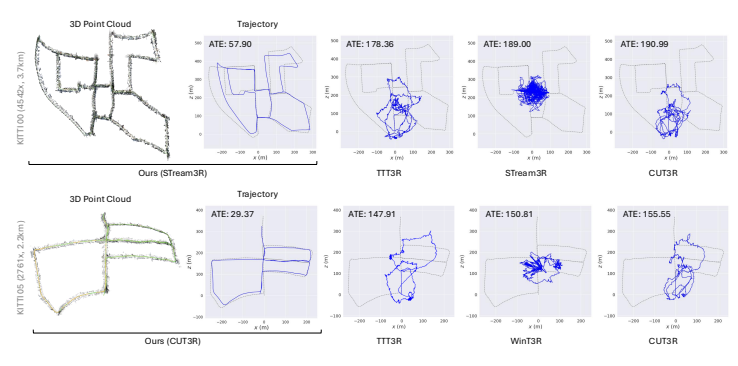Qualitative trajectory comparison on KITTI long sequences.

Figure 7: Qualitative trajectory comparison on KITTI long sequences. [235]

4.4. Ablation Study [217]

Ablation studies are conducted on vKITTI and KITTI to validate key components of the method. [217] These cover model training strategy, inference-time design choices, and loop closure. [218] Results are summarized in Tables 5 to 7. [218]

Model Training Strategy [219]
1. Removing reference-frame supervision entirely (w/o reference) sharply degrades RPEtrans to 3.336 (Table 5). [219]
2. A single reference reduces ATE to 15.764. [230]
3. The full multi-reference training achieves the best ATE of 5.632. [230]
4. This confirms that denser reference supervision is critical for robust long-sequence pose estimation. [230]
Method ATE ↓ RPEtrans ↓ RPErot ↓

Baseline (CUT3R) 56.390 1.678 0.342

w/o reference 33.318 3.336 0.842

1 reference 15.764 0.217 0.448

Ours 5.632 0.177 0.485

Table 5: Ablation on training strategy (vKITTI). Denser reference supervision consistently lowers ATE, while removing references entirely causes severe RPE degradation. [225]
Inference-Time Components [231]
1. Table 6 ablates the inference-time pipeline. [231]
2. Removing keyframe selection or PGO each leaves a large gap to the full system (ATE: 38.258 without keyframe selection). [231]
3. Progressively increasing reference count from 4 to 12 consistently reduces ATE from 15.748 to 5.632. [232]
Method ATE ↓ RPEtrans ↓ RPErot ↓

w/o keyframe 38.258 0.787 1.388

w/o PGO 20.089 0.203 0.544

K = 4 15.748 0.188 0.470

K = 8 7.362 0.180 0.470

Full (K = 12) 5.632 0.177 0.485

Table 6: Ablation on inference time components (vKITTI). Both keyframe selection and PGO are essential, and scaling the reference count from 4 to 12 at inference time consistently reduces ATE without retraining. [225]
Runtime Analysis [234]
1. Figure 15 breaks down the latency on KITTI (K=12). [234]
2. The frozen forward pass dominates on both backbones (86.3% on CUT3R, 91.2% on STream3R). [234]
3. Keyframe selection, PGO, and loop detection add little overhead. [235]
4. The full pipeline runs at 14.4 and 7.95 FPS, versus 15.9 and 9.1 FPS for the backbones. [235]

Method	ATE ↓	RPEtrans ↓	RPErot ↓
Baseline (CUT3R)	56.390	1.678	0.342
w/o reference	33.318	3.336	0.842
1 reference	15.764	0.217	0.448
Ours	5.632	0.177	0.485

Method	ATE ↓	RPEtrans ↓	RPErot ↓
w/o keyframe	38.258	0.787	1.388
w/o PGO	20.089	0.203	0.544
K = 4	15.748	0.188	0.470
K = 8	7.362	0.180	0.470
Full (K = 12)	5.632	0.177	0.485

Loop Closure [242]

As shown in Table 7 and Figure 10, loop closure reduces average ATE on KITTI from 143.45 to 75.01 (48% improvement). [242]
This has particularly large gains on sequences containing large loops (e.g., Seq. 00 and Seq. 05). [243]
Globally consistent trajectory correction is most needed in these sequences. [243]

Method	LC	Avg.	00	02	05	06	07	08	09
Ours (CUT3R)		143.45	185.70	235.28	108.73	84.86	49.83	241.86	97.86
	✓	75.01	45.34	139.88	29.37	47.40	6.44	227.02	29.63
Ours (STream3R)		129.40	166.37	239.36	134.08	35.95	60.68	195.20	74.18
	✓	78.39	57.90	170.75	39.05	18.07	15.19	173.83	73.91

Table 7: Ablation on loop closure (KITTI, ATE ↓). Loop closure reduces average ATE by 48%, with the largest gains on loop-heavy sequences. [239]

Robustness Analysis [244]
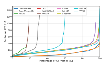
1. Figure 9 presents per-frame ATE curves sorted in ascending order across all KITTI sequences. [244]
2. Methods such as MUSt3R and Point3R suffer catastrophic failures at moderate sequence lengths. [244]
3. Scal3R maintains the lowest per-frame ATE throughout the entire evaluation range. [245]
4. This confirms superior robustness under challenging long-sequence conditions. [245]

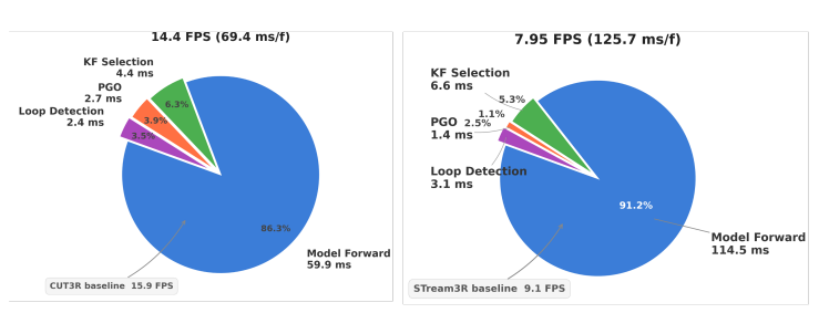Per-frame runtime breakdown on KITTI.

Figure 8: Per-frame runtime breakdown on KITTI. [248]

Robustness Analysis on KITTI.

Figure 9: Robustness Analysis on KITTI. [252]

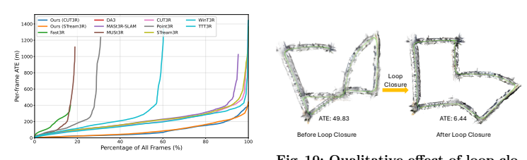Qualitative effect of loop closure on KITTI 07.

Figure 10: Qualitative effect of loop closure on KITTI 07. [256]

5. Conclusion [246]

Scal3R addresses the instability of global pose regression on long sequences. [246] It reformulates camera localization as multi-reference relative pose querying on a frozen backbone. [247]

Key features and performance [259]
1. Lightweight tokens (~1% of parameters) query relative poses. [259]
2. An online pose-graph backend aggregates these into a globally consistent trajectory. [260]
3. Trained in 8 hours on a single GPU, Scal3R enables accurate online reconstruction of long video streams. [260]
Limitations [261]
1. Performance is bounded by the frozen backbone, degrading under occlusion or textureless regions. [261]
2. The online backend has its own weaknesses. [262]
  1. Appearance-based loop closure can miss revisits under extreme viewpoint or illumination change. [262]
  2. Keyframe selection and loop detection rely on hand-set thresholds. [263]
3. Improving both remains future work. [263]

Just add sources; your living note is ready

Fully trustworthy notes with source links

A variety of notes tailored to your goals

AI chat grounded in your uploaded sources

Deep Search that finds trustworthy sources