QCell: Recombining and Aligning Cell Queries for Overlapping Instance Segmentation

0. Abstract

arXiv:2608.29253 · Yaroslav Prytula, Anton Popov, Dmytro Fishman


Core	A query-based model for de-overlapping cell instance segmentation in microscopy.
Gap	Existing methods lack global reasoning for semi-transparent, overlapping cell structures.
Approach	Instance recombination of amodal/visible/invisible sub-queries + contrastive query alignment.
Result	Outperforms state-of-the-art with +2.2 AP and +2.7 AJI on ISBI2014.

The Question — How can a query-based model effectively segment overlapping cells in microscopy images, especially given weak boundaries and mixed visual evidence? [4]

Instance segmentation of overlapping cells in microscopy is challenging. [4]
1. This is due to semi-transparent structures. [4]
2. These structures produce weak boundaries and mixed visual evidence in overlap regions. [4]
Existing methods use local regions of interest or shape priors. [5]
1. However, these methods lack global reasoning across overlapping objects. [5]
QCell is a novel query-based model. [6]
1. It de-overlaps cell instances in microscopy scenes. [6]
2. QCell combines two main components: [6]
  1. An instance recombination module. [6]
    1. This module decomposes and recombines query representations in latent space. [6]
    2. It enables the model to reason about complete object structure under overlap. [7]
  2. A contrastive query alignment objective. [7]
    1. This objective combines distinctive instance feature learning. [7]
    2. It also separates overlapping cell queries. [8]
The authors introduce a new Organoid dataset benchmark. [8]
1. This dataset is for overlapping cell segmentation. [9]
QCell outperforms state-of-the-art methods across multiple benchmarks. [9]
1. It achieves +2.2 AP and +2.7 AJI on ISBI2014. [9]

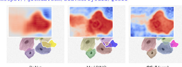QCell vs. other methods on overlapping cells

Figure 1. QCell better preserves complete structures and separates neighboring instances compared to DoNet and MaskDINO. [10]

1. Introduction

Cell instance segmentation is a fundamental step in microscopy image analysis. [19]

It enables downstream measurements of: [19]
1. Cellular morphology. [20]
2. Spatial organization. [20]
3. Population-level behavior. [20]
This task is challenging across various imaging modalities. [20]
1. Challenges include non-specific contrast, high cell morphology variability, noise, and unclear boundaries. [21]
In dense cultures, cells often form overlapping clusters. [22]
1. Unlike natural-image occlusion where regions are visually absent, microscopy often shows semi-transparent overlap. [22]
2. Hidden cell structures remain partially visible but with weak contrast and mixed visual evidence. [23]
3. Overlapping regions contain information from multiple instances. [24]
4. This produces ambiguous boundaries and strong appearance entanglement between neighboring cells. [24]

1.1. Resolving Overlapping Instances [25]

Resolving overlapping instances requires amodal reasoning. [25]
1. This means understanding the complete object extent from partial observations. [25]
Existing approaches [26]
1. They use region-level decomposition, shape priors, or multi-stage generative completion. [26]
2. These methods typically operate on local Region of Interest (RoI) features. [27]
3. They also depend on upstream predictions. [27]
4. This limits their ability to jointly reason over the full scene. [27]
For overlapping cells, understanding inter-instance relationships is essential. [27]
1. This helps determine which evidence belongs to which cell. [28]
Query-based segmentation models [28]
1. These models are a natural fit for this problem. [28]
2. Each instance is represented by a query. [29]
3. The query attends globally to image features. [29]
4. It interacts with all other queries. [29]
5. This enables inter-instance communication needed for reasoning about shared overlap regions in the full scene context. [29]

1.2. QCell Approach [30]

QCell is designed for overlapping cell instance segmentation. [30]
De-overlapping requires understanding object structure in terms of visible and hidden parts. [31]
Instance Decomposition and Recombination [31]
1. Each instance query is decomposed into amodal, visible, and invisible sub-representations. [31]
2. These are recombined with consistency regularization. [32]
3. This improves complete object perception. [32]
Contrastive Query Learning [32]
1. This ensures queries of overlapping cells remain distinguishable. [32]
2. It leverages denoising queries. [33]
3. Denoising queries provide stable ground-truth-initialized representations during training. [33]
4. It combines an instance discriminative loss with a query alignment loss. [33]
5. This separates queries in embedding space. [34]

1.3. Contributions [34]

Query-level instance decomposition and recombination [35]
1. This includes consistency regularization. [35]
2. It models amodal, visible, and invisible cell structure. [35]
DN-guided contrastive query learning [36]
1. This uses instance-discriminative and cosine alignment losses. [36]
2. It improves the separation of overlapping cells. [36]
New Organoids benchmark [37]
1. This benchmark evaluates overlapping cell instance segmentation. [37]

2. Related Work

Segmenting overlapping instances requires reasoning about object structure and inter-instance relationships. [38]

Prior works have explored these problems from different angles. [38]

2.1. Amodal Instance Segmentation [40]

Instance segmentation has primarily been built on two-stage detection frameworks. [40]
1. Mask R-CNN introduced a mask prediction head on top of Faster R-CNN. [41]
2. Subsequent methods like Cascade R-CNN and HTC refined the multi-stage pipeline. [41]
3. These models form the foundation for overlapping and amodal segmentation methods. [42]
Direct methods [43]
1. These are occlusion-aware extensions of the two-stage pipeline. [43]
2. They introduce dedicated modules for handling overlapping instances. [43]
3. Occlusion R-CNN adds a bilayer decoupling head. [44]
  1. This head separates occluder and occludee representations within each RoI. [44]
  2. It predicts visible and amodal masks. [45]
4. BCNet predicts two overlapping layers via graph convolutional networks on RoI features. [45]
5. Another method formulates overlap as a depth-ordering problem. [46]
  1. It assigns layer indices to instances through a U-Net architecture. [47]
6. AISFormer uses transformer queries in the RoI pipeline. [47]
  1. It introduces mask tokens for occluder, visible, amodal, and invisible types. [47]
  2. These tokens interact through self-attention. [48]
7. For cytology, DoNet uses a decompose-and-recombine strategy. [48]
  1. It decomposes cell clusters into intersection and complement regions. [48]
  2. This is done through a Dual-path Region Segmentation Module. [49]
  3. It is followed by consistency-guided recombination. [49]
8. GAInS generates gradient anomaly maps. [49]
  1. These maps capture spatial regions of crossing, touching, and overlapping. [50]
  2. They are used to reweight the mask prediction loss in error-prone overlap regions. [50]
Shape-prior methods [51]
1. These approaches learn object shape distributions to complete occluded regions. [51]
2. C2F-Seg and ShapeFormer learn latent shape representations for coarse-to-fine amodal mask refinement. [52]
3. Prior-Guided Expansion retrieves regression and flow transformations from a memory bank of shape priors. [52]
4. ShapeMoE routes each instance to a specialized expert based on learned Gaussian shape embeddings. [53]
5. VRSP-Net employs a diffusion-based shape prior estimation module conditioned on visible features. [54]
6. These methods assume a learnable shape distribution. [55]
  1. This becomes problematic for cells with extreme morphological diversity. [55]
Generative methods [56]
1. Diffusion-based approaches have been applied to amodal completion. [56]
2. pix2gestalt uses conditional diffusion to synthesize complete objects from partial observations in a zero-shot manner. [57]
3. MC Diffusion separates query objects from occluding context. [57]
  1. It applies progressive mixed-context diffusion for amodal completion. [58]
4. SAS formulates sequential amodal segmentation. [58]
  1. This is done through cumulative occlusion learning. [58]
  2. It predicts amodal masks layer-by-layer from unoccluded to deeply occluded objects. [59]
5. These methods depend on upstream visible mask quality as conditioning input. [59]
  1. This creates pipeline dependencies where segmentation errors propagate. [59]
Foundation model adaptation [59]
1. SAMBA proposes a SAM-based amodal segmentation foundation model. [59]
  1. It uses a separation-to-fusion structure for joint modal and amodal prediction. [60]
2. SAMEO adapts the Segment Anything model for occluded scene understanding. [60]
3. These approaches must acquire overlap-handling behavior from data alone. [61]
  1. They lack explicit de-overlapping objectives. [61]
  2. This requires large curated amodal datasets, which are scarce in biomedical domains. [61]

2.2. DETR Models [63]

DETR reformulated object detection as a set prediction problem. [63]
1. Learnable queries attend to image features through a transformer decoder. [63]
Improvements to DETR [64]
1. Deformable DETR improved efficiency with multi-scale deformable attention. [64]
2. DN-DETR introduced denoising training. [65]
  1. It injected noise-perturbed ground-truth labels as additional queries for reconstruction. [65]
  2. This improved convergence. [66]
3. DINO extended this idea with contrastive denoising groups and mixed query selection. [66]
4. Mask2Former introduced masked attention. [67]
  1. This restricted cross-attention to predicted foreground regions for segmentation. [67]
5. MaskDINO unified detection and segmentation. [68]
  1. It added mask prediction through query-pixel dot products. [68]
  2. It inherited denoising training. [69]
Advantages of query-based architectures [69]
1. Unlike region-based methods, they allow each query to attend globally over the full image. [69]
2. This enables inter-instance communication for reasoning about overlapping objects. [70]
Biomedical domain applications [71]
1. IAUNet introduces a query-based U-Net architecture. [71]
  1. It has a lightweight convolutional Pixel decoder and a Transformer decoder. [72]
  2. It refines object-specific features across multiple scales. [72]
  3. It shows strong performance in cell segmentation. [72]
2. PCTrans uses position-guided cross-attention and contrastive losses on query embeddings. [73]
  1. This learns discriminative representations in dense biological scenes. [73]
  2. However, it primarily targets crowded instances without explicit modeling of overlapping object structure. [74]
Failure modes in dense scenes [75]
1. Mask transformers exhibit specific failure modes in dense scenes. [75]
2. DAC-DETR shows that cross-attention gathers multiple queries toward the same object. [76]
  1. Self-attention disperses them to avoid duplicates. [76]
  2. Learning these opposing effects jointly becomes difficult when nearby objects create conflicting signals. [76]
3. PanSR demonstrates instance merging. [77]
  1. Distinct objects collapse into one mask. [77]
  2. It addresses this by constraining mask predictions with bounding box geometry. [78]

2.3. Contrastive Learning for Instance Discrimination [79]

In overlapping scenes, learning discriminative instance representations is essential. [79]
1. This helps distinguish objects that share similar appearance and spatial context. [80]
Contrastive learning provides a natural framework for shaping these representations. [80]
Category-level contrastive learning [81]
1. This has focused primarily on category-level query discrimination for DETR-based detectors. [81]
2. CSPCL aligns content queries with category prototypes. [81]
  1. It uses intra-class attraction and inter-class repulsion losses. [82]
  2. This corrects missing semantic information for prohibited item detection in overlapping X-ray images. [82]
3. MMCL proposes a multi-class min-margin contrastive loss for anti-overlapping X-ray detection. [83]
  1. It balances intra-class diversity with inter-class separability. [83]
4. These methods improve category discrimination. [84]
  1. However, they do not address same-class instance separation. [84]
  2. This is the primary challenge in cell segmentation, where all overlapping objects belong to the same category. [84]
Instance-level contrastive learning [85]
1. This has been explored primarily in video instance segmentation. [85]
  1. Temporal association provides natural positive and negative pairs. [85]
2. CAVIS uses prototypical cross-frame contrastive loss. [86]
  1. This maintains instance embedding consistency across frames. [86]
3. VISAGE employs appearance-guided contrastive objectives for instance identity preservation across video frames. [86]
4. MDQE mines discriminative query embeddings for video segmentation under occlusion. [87]
  1. This is done through temporal cross-attention and inter-instance mask repulsion. [88]
5. ConQueR and similar methods embed ground-truth instances into the query space for contrastive training. [88]
  1. This reduces false positive predictions in 3D detection. [89]
6. These methods form contrastive pairs from temporal correspondences or ground-truth embeddings. [89]
  1. They do not impose explicit geometric constraints on pairwise similarity structure needed for de-overlapping. [90]
7. QCell combines discriminative feature learning with cosine alignment. [90]
  1. This ensures queries of overlapping cells remain well-separated in the embedding space. [91]

3. Method

QCell addresses overlapping cell instance segmentation. [92]

It extends MaskDINO with complementary objectives. [92]
These objectives target object structure modeling and query discrimination in dense overlap scenes. [93]

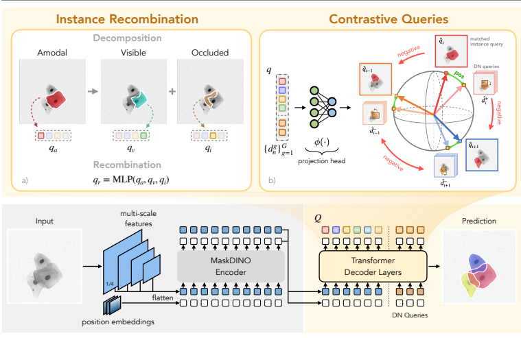QCell Overview Diagram

Figure 2: Overview of QCell. QCell builds on a MaskDINO-style query-based segmentation pipeline. [89]

3.1. Preliminaries: MaskDINO [94]

MaskDINO Overview — MaskDINO is a unified query-based framework for detection and segmentation. [95] It extends DINO with a mask prediction branch. [95]

Architecture [96]
1. A backbone network extracts multi-scale features from an input image. [96]
2. A pixel decoder processes these features to produce multi-scale feature maps {Fl} and a high-resolution pixel embedding map F. [96]
3. A set of N learnable content query embeddings Q is iteratively refined. [97]
  1. This happens through a stack of transformer decoder layers. [98]
  2. Each layer consists of self-attention among queries, multi-scale deformable cross-attention with feature maps, and a feed-forward network. [98]
4. After decoding, parallel prediction heads produce: [99]
  1. Per-query classification scores cn. [99]
  2. Bounding box coordinates bn. [100]
  3. Instance masks Mn, obtained via dot product Mn = q⊤n F. [100]
5. During training, the Hungarian algorithm assigns M predictions to ground-truth instances. [100]
  1. This is done through one-to-one bipartite matching. [101]
  2. Remaining N − M queries are assigned to the "no object" class. [101]
DeNoising (DN) training [102]
1. The decoder also receives DN queries. [102]
2. These are constructed by adding random noise to ground-truth bounding boxes and class labels. [102]
3. They are organized into G denoising groups. [103]
  1. Each group contains a noised version of all M instances. [103]
4. The DN query for instance n in group g is denoted as dng. [103]
5. The decoder reconstructs clean targets from these noisy initializations. [104]
  1. This accelerates convergence. [104]
6. In QCell, DN queries are repurposed as stable anchors for contrastive learning. [104]
Standard MaskDINO training objective [105] $L_{ba se} = λ_{c l s} L_{c l s} + λ_{b o x} L_{b o x} + λ_{ma s k} L_{ma s k} + L_{d n} . (1)$
Limitations in overlapping cell segmentation [106]
1. The single mask prediction does not model the relationship between visible and occluded object parts. [106]
2. The training objective lacks explicit supervision for learning discriminative instance features in dense overlapping scenes. [107]

3.2. Instance Recombination [108]

Core Idea — The Instance Recombination module brings the decompose-and-recombine principle to the query level. [109] This removes dependency on region proposals and enables global attention reasoning about object structure. [110]

When semi-transparent cells overlap, the intersection region contains blended visual signals from both instances. [108]
Standard segmentation models produce a single mask per instance. [108]
1. This makes it difficult to learn complete object structure. [109]
2. This is due to limited perception capability in overlapping regions. [109]
3. Parts of the object are shared with or hidden by neighboring cells. [109]
Decomposition [111]
1. For each content query embedding q in the decoder, three lightweight MLP heads produce sub-query representations. [111]
2. These correspond to structural components of an instance: [112]
  $q_{k} = M L P_{k} (q), k \in {a, v, i}, (2)$
  1. qa encodes the amodal (full extent) representation. [113]
  2. qv encodes the visible (non-overlapped part) representation. [113]
  3. qi encodes the invisible (occluded part) representation. [113]
3. Each sub-query generates its corresponding mask. [114]
  1. This is done through a dot product with the pixel features F: [114] $M_{k} = q_{k}^{⊤} F, k \in {a, v, i} . (3)$
4. All queries in the decoder pass through the decomposition heads. [114]
5. During training, matched queries are supervised with corresponding ground-truth component masks. [115]
6. Each sub-mask is supervised with binary cross-entropy and dice losses: [115]
  $L_{d eco m p} = k \in {a, v, i} \sum [L_{b ce} (M_{k}, G_{k}) + L_{d i ce} (M_{k}, G_{k})], (4)$
  1. Ga, Gv, Gi are the ground-truth amodal, visible, and invisible masks. [117]
Recombination [118]
1. After decomposition, sub-query representations are recombined to produce a refined full-instance embedding. [118]
2. The three sub-queries are fused through a learned projection: [119]
  $q_{r} = M L P (q_{a}, q_{v}, q_{i}), (5)$
  1. This integrates information from all structural components into a single refined representation. [120]
3. The refined mask Mr is obtained as Mr = q⊤r F. [120]
  1. It is supervised against the full amodal ground truth Ga: [120] $L_{r e f in e d} = L_{b ce} (M_{r}, G_{a}) + L_{d i ce} (M_{r}, G_{a}) . (6)$
4. The recombination step encourages sub-queries to capture complementary information. [121]
  1. Their fusion must recover the complete object. [122]
5. The refined query embedding qr encodes richer structural knowledge. [122]
  1. It is trained to reason about both visible and hidden regions. [123]
Consistency regularization (CR) [123]
1. A consistency regularization loss enforces geometric coherence. [123]
  1. This is between decomposed parts and the recombined prediction. [124]
2. The key constraint is that the refined mask should be recoverable from the union of visible and invisible predictions: [124]
  $L_{C R} = L_{b ce} (M_{r}, s g [X O R (σ (M_{v}) > 0.5, σ (M_{i}) > 0.5)]), (7)$
  1. σ is the sigmoid function. [125]
  2. sg(·) denotes the stop-gradient operator. [125]
  3. XOR(·,·) produces the recombined binary mask from thresholded visible and invisible predictions. [125]
  4. The binary mask is treated as a fixed pseudo-target. [125]
  5. Gradients from LCR flow only through the refined prediction Mr. [125]
3. The recombination loss is: [125] $L_{r eco mb} = L_{r e f in e d} + L_{C R} . (8)$
4. The complete instance recombination loss is: [125] $L_{I R} = L_{d eco m p} + L_{r eco mb} . (9)$

3.3. Contrastive Query Learning [126]

Core Idea — This module addresses representational similarity between queries of overlapping instances. [126] It decouples the contrastive objective into two requirements: distinctive instance features and separation of co-occurring instances. [128]

The instance recombination module provides structural supervision. [126]
1. However, it does not address representational similarity between queries of overlapping instances. [127]
Under heavy overlap, content query embeddings of nearby cells converge through self-attention. [127]
1. This leads to representational collapse. [128]
QCell addresses this through contrastive losses on query embeddings within each decoder level. [129]
DeNoising queries as stable anchors [130]
1. DN queries provide a natural foundation for contrastive learning. [130]
2. Each ground-truth instance is guaranteed G DN representations {dng}Gg=1. [130]
  1. This is regardless of matching quality. [131]
  2. They serve as reliable anchors. [131]
3. Their stability over matched queries is empirically confirmed in Tab. 5. [131]
Contrastive projection [132]
1. A lightweight projection head φ maps content query embeddings into a shared contrastive space. [132]
2. Both DN queries and matched queries are projected through φ. [133]
  1. This produces normalized embeddings. [133]
3. The projected matched query for instance n is denoted as ˆqn = φ(qn). [134]
4. The projected DN query for instance n in group g is denoted as dˆng = φ(dng). [134]
5. For each projected matched query ˆqn: [134]
  1. The positive set Pn = {dˆng}Gg=1 consists of all denoising DN embeddings for the same instance across groups. [135]
  2. The negative set Nn = {dˆjg | j ̸= n, g ∈ {1,...,G}} consists of DN embeddings for all other instances. [135]
Instance-discriminative loss [136]
1. An InfoNCE-based objective encourages the model to learn discriminative instance features. [137]
2. Using ˆqn as the anchor, Pn as positives, and Nn as negatives: [137]
  $L_{d i sc} = - n = 1 \sum M lo g \frac{\sum _{k^{+} \in P_{n}} exp ( q ^ _{n} \cdot k ^{+} / τ )}{\sum _{k^{+} \in P_{n}} exp ( q ^ _{n} \cdot k ^{+} / τ ) + \sum _{k^{-} \in N_{n}} exp ( q ^ _{n} \cdot k ^{-} / τ )} . (10)$
  1. M is the number of matched instances. [139]
  2. τ is a temperature parameter. [139]
3. This loss encourages each matched query to learn discriminative features. [139]
  1. These features align with its corresponding DN representations. [140]
  2. They remain distinct from DN representations of other instances. [140]
Latent alignment loss [141]
1. This loss complements the contrastive objective. [141]
2. It imposes direct geometric constraints on the embedding space. [142]
3. It uses the same positive and negative sets Pn and Nn: [142] $L_{a l i g n} = n = 1 \sum M [k^{+} \in P_{n} \sum (cos (\overset{q}{^}_{n}, k^{+}) - 1)^{2} + k^{-} \in N_{n} \sum cos (\overset{q}{^}_{n}, k^{-})^{2}] . (11)$
4. The first term pulls matched predictions toward their corresponding DN representations across denoising groups. [149]
  1. This reinforces identity consistency. [150]
5. The second term pushes matched predictions toward orthogonality with DN representations of other instances. [150]
  1. This directly penalizes high cosine similarity that leads to representational collapse. [151]
6. Both losses are applied across multiple decoder layers. [151]

3.4. Training Objective [158]

The complete training objective combines baseline MaskDINO losses with the three proposed components: [158] $L = L_{ba se} + λ_{I R} L_{I R} + λ_{d i sc} L_{d i sc} + λ_{a l i g n} L_{a l i g n} . (12)$
Losses are computed on each decoder layer and summed. [160]
1. This follows the auxiliary loss strategy in DETR-based architectures. [160]
Weighting parameters [160]
1. λcls = 4.0, λbce = 5.0, λdice = 5.0, λbox = 5.0, and λgiou = 2.0. [160]
2. For Instance Recombination: [161]
  1. Coarse mask BCE and Dice losses are weighted by 5.0. [161]
  2. Consistency loss is weighted by 1.0. [162]
3. For contrastive objective: [162]
  1. λdisc = 2.0 and λalign = 5.0. [162]
  2. Temperature τ = 0.1. [163]

4. Experiments

This section evaluates QCell on multiple datasets. [164]

This includes the novel Organoids benchmark for overlapping cell segmentation. [164]
It provides comprehensive comparisons with state-of-the-art methods. [165]
Ablation studies demonstrate the effectiveness of each model component. [165]
Evaluation is on three microscopy datasets that pose overlapping challenges: [166]
1. They range in fine-grained details and object count. [167]
2. They cover different imaging modalities. [167]

4.1. Datasets [168]

ISBI2014 [168]
1. This dataset is from the Overlapping Cervical Cytology Image Segmentation Challenge. [168]
2. It includes 16 real extended depth-of-focus (EDF) cervical cytology images. [169]
3. It also has 945 synthetic images. [169]
4. Images have high-quality pixel-level annotations for nuclei and cytoplasm at 512×512 resolution. [170]
5. The challenge setting uses 45 synthetic images for training, 90 for validation, and 810 for testing. [170]
6. The focus is on overlapping objects. [171]
7. All models are benchmarked on cytoplasm annotations only. [171]
  1. This is where semi-transparent overlap between cells is most prevalent. [172]
Revvity-25 [172]
1. It consists of 110 high-resolution 1080×1080 brightfield images. [172]
2. Each image contains an average of 27 manually labeled and expert-validated cancer cells. [173]
3. This totals 2,937 annotated instances. [173]
4. The dataset provides highly accurate and detailed annotations for cell borders and overlap regions. [173]
5. This makes it a challenging benchmark for precise boundary delineation in dense scenes. [174]
Organoids [175]
1. This is a novel Organoids dataset for overlapping object segmentation in brightfield microscopy. [175]
2. The dataset contains 1,186 training images, 1,199 validation images, and 201 test images. [175]
3. Images are at a resolution of 540 × 540. [176]
4. It presents dense and highly overlapping scenes. [176]
  1. Up to 105 instances per training image. [177]
  2. An average of 96 instances per test image. [177]
  3. A maximum of 223 instances. [177]
5. This makes Organoids a challenging real-world benchmark for evaluating instance separation and de-overlapping. [177]
6. Additional dataset details are in the Supplementary Material. [178]

4.2. Implementation Details [179]

Experimental Setup — 1. Model Implementations: Detectron2-based for all experiments. [179]

Backbone: ResNet-50-FPN with ImageNet-pretrained weights. [179]
Mask Prediction: All models trained to predict full amodal masks. [180]
Optimizer: [180]
1. R-CNN-based models: SGD with momentum 0.9. [180]
  1. Initial learning rate: 10−3. [181]
  2. Linear warm-up during first 1k iterations. [181]
2. Query-based models: AdamW with initial learning rate 10−4 and weight decay 0.05. [182]
  1. Backbone learning-rate multiplier: 0.1. [183]
Queries: [182]
1. ISBI2014 and Revvity-25: 100 queries. [182]
2. Organoids: 300 queries. [182]
Training Schedule: [183]
1. All models trained for 60k iterations. [183]
2. Batch size: 2. [184]
3. Learning rate decreased by 0.1 at 50k and 55k iterations. [184]
Checkpoint Selection: Best checkpoint based on validation-set performance. [184]
Reporting: Test results averaged over three random seeds. [185]
Evaluation Protocol: Same for all methods. [185]
Hardware: Single NVIDIA H200 Tensor Core GPU with 141 GB HBM3e memory. [185]

4.3. Main Results [186]

QCell is compared with state-of-the-art amodal and cell instance segmentation methods. [186]
1. This is done on ISBI2014, Revvity-25, and Organoids. [187]

Models	AP	AP50	AP75	DICE	F1	AJI	#params.	FLOPs
Mask R-CNN [11]	55.6	84.0	58.9	91.2	88.1	72.4	44M	128G
ORCNN [42]	60.6	86.3	65.3	92.0	90.0	75.4	46M	132G
VRSP-Net [39]	51.1	81.6	53.4	91.6	88.5	73.1	99M	118G
BCNet [15]	47.6	77.8	48.3	56.6	53.6	41.1	38M	308G
AISFormer [35]	55.5	84.9	58.7	90.9	88.9	73.0	45M	130G
PCTrans† [7]	15.4	34.6	11.9	87.3	56.3	40.2	31M	99G
GAInS [25]	54.8	83.9	59.0	90.9	89.0	73.0	53M	117G
DoNet [14]	60.9	86.2	66.1	92.1	89.6	75.2	73M	117G
Mask2Former [8]	56.3	83.1	56.2	90.7	88.2	71.1	44M	159G
MaskDINO [20]	63.7	89.0	65.4	92.3	90.0	75.9	44M	163G
QCell (ours)	65.9	91.9	69.1	92.4	92.3	78.6	45M	182G

Table 1: Comparison on ISBI2014 and Revvity-25. QCell achieves the best overall performance on both benchmarks, improving AP and AJI over prior amodal and cell instance segmentation methods. [140]

ISBI2014 cytoplasm segmentation [187]
1. QCell achieves the best performance. [187]
  1. 65.9 AP, 92.3 F1, and 78.6 AJI. [188]
2. Compared to MaskDINO baseline, QCell improves: [188]
  1. AP by +2.2. [189]
  2. F1 by +2.3. [189]
  3. AJI by +2.7. [189]
3. QCell produces more object-consistent masks. [189]
  1. This is especially true where neighboring cells share weak or semi-transparent boundaries. [190]
4. Two-stage R-CNN-based methods struggle to segment highly overlapping instances. [190]
  1. QCell better preserves separated object masks in these cases. [191]
Revvity-25 [192]
1. QCell also achieves the best AP and AJI. [192]
  1. 52.9 AP, 86.4 F1, and 73.6 AJI. [193]
2. The model produces visually cleaner segmentations with fewer false positives in dense regions. [193]
3. Query-based models preserve fine cell structures better than R-CNN-based methods. [194]
  1. R-CNN methods often miss thin boundaries or merge nearby instances under strong overlap. [195]

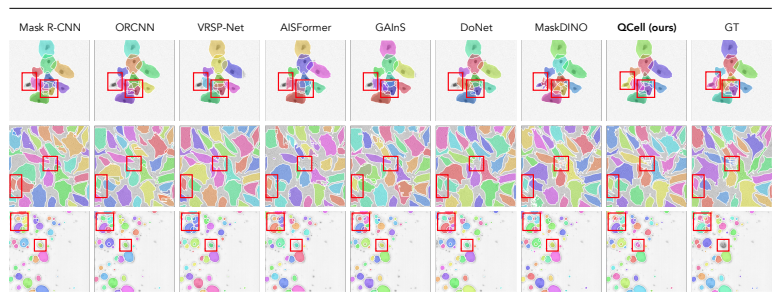Qualitative comparison of QCell across datasets

Figure 3: Qualitative comparison across datasets. QCell produces more object-consistent instance masks across ISBI2014, Revvity-25, and Organoids. [171]

Models	AP	AP50	AP75	DICE	F1	AJI	#params.	FLOPs
Mask R-CNN [11]	50.6	68.7	55.9	93.9	68.6	61.7	44M	128G
ORCNN [42]	48.7	67.1	54.3	93.4	70.6	62.4	46M	132G
VRSP-Net [39]	50.3	67.6	55.7	93.0	72.3	62.6	99M	118G
BCNet [15]	50.3	67.7	55.3	94.1	62.7	58.6	38M	308G
AISFormer [35]	49.5	67.7	55.1	93.7	66.9	60.4	45M	130G
PCTrans† [7]	11.7	28.1	8.1	86.0	50.4	40.9	31M	99G
GAInS [25]	48.8	67.1	54.4	93.5	66.6	59.9	53M	117G
DoNet [14]	50.5	67.7	55.8	94.2	66.8	61.0	73M	117G
Mask2Former‡ [8]	34.7	47.2	38.4	92.3	63.3	54.2	44M	159G
Mask2Former [8]	31.3	46.9	33.9	91.0	48.2	36.2	44M	185G
MaskDINO [20]	49.7	68.7	54.7	92.2	71.5	63.1	44M	163G
QCell (ours)	51.0	69.1	56.4	92.5	71.6	63.2	45M	182G

Table 2: Comparison on Organoids. QCell achieves the best overall results on the Organoids dataset. [157]

Organoids [195]
1. QCell remains competitive in this densely populated benchmark. [195]
2. It achieves the best overall results. [196]
  1. 51.0 AP, 71.6 F1, and 63.2 AJI. [197]
3. The dataset contains substantially more instances per image than ISBI2014 and Revvity-25. [197]
  1. This makes accurate instance ranking and separation more difficult. [197]
4. QCell achieves the best AP and AJI among compared methods. [198]
  1. This shows that the proposed query-based de-overlapping strategy generalizes to high-density microscopy scenes. [198]
Mask2Former on Organoids [199]
1. Mask2Former trained with N = 100 and N = 300 object queries is reported. [199]
2. The N = 300 configuration matches the query count used by other query-based models. [200]
3. The N = 100 configuration is retained because increasing queries degraded Mask2Former performance. [200]
PCTrans mask representation [201]
1. PCTrans differs from other instance segmentation methods in its mask representation. [201]
2. The framework predicts categorical masks. [202]
  1. Each pixel receives a single label. [202]
3. PCTrans shows limited generalization to overlapping amodal cell segmentation. [202]
4. It obtains reasonable F1 and AJI scores. [203]
5. AP stays low because the model does not produce per-instance confidence scores. [203]
  1. Thus, AP has no meaningful ranking. [203]

5. Ablation Studies

This section ablates the main components of QCell on ISBI2014. [204]

5.1. Instance Recombination [205]

Impact of Instance Recombination — The Instance Recombination (IR) module improves complete object reasoning under overlap. [205] It decomposes queries into amodal, visible, and invisible sub-representations and recombines them. [206]

Lbase	Ldecomp	Lrecomb	Ldisc	Lalign	AP	AP50	AP75	DICE	F1	AJI
✓					63.7	89.0	65.4	92.3	90.0	75.9
✓	✓				65.1	89.8	68.1	92.6	90.0	76.2
✓	✓	✓			66.6	90.1	69.2	92.8	90.7	77.1
✓			✓		65.5	89.8	67.5	92.6	90.6	76.7
✓				✓	66.2	89.7	68.6	92.6	90.5	76.4
✓			✓	✓	67.0	91.0	69.2	92.7	91.6	77.9
✓	✓	✓	✓	✓	65.9	91.9	69.1	92.4	92.3	78.6

Table 3: Ablation study on ISBI2014. Lbase denotes the standard MaskDINO objective, Ldecomp the decomposition loss, Lrecomb = Lrefined + LCR the recombination loss, Ldisc the instance-discriminative loss, and Lalign the cosine alignment loss. [189]

Adding the instance recombination loss improves the MaskDINO baseline. [206]
1. AP increases from 63.7 to 65.1. [207]
2. AP75 increases from 65.4 to 68.1. [207]
Adding Consistency Regularization (CR) further improves performance. [208]
1. It reaches 66.6 AP, 69.2 AP75, and 77.1 AJI. [208]
2. Enforcing consistency between visible, invisible, and recombined full masks helps produce more coherent object predictions in overlapping regions. [209]

5.2. Contrastive Query Learning [212]

Impact of Contrastive Query Learning — In overlapping regions, object features from neighboring cells mix, making it difficult for queries to learn distinctive instance representations. [212] Contrastive Query Learning addresses this by improving query representations. [213]

DN oracle analysis [213]
1. Main-query predictions are matched to ground-truth instances using the Hungarian matcher. [214]
2. They are then replaced with corresponding DN-query predictions at test time. [214]
3. The mean performance over all DN queries across three random seeds is reported. [214]
4. This improves performance from 63.7 to 68.6 AP and from 75.9 to 80.0 AJI. [215]
5. This suggests that DN queries capture higher-quality instance representations. [215]
6. This motivates their use as supervision anchors for contrastive query learning. [216]
Effect of each contrastive loss [216]
1. Adding Ldisc alone improves the baseline to 65.5 AP. [216]
2. Lalign alone reaches 66.2 AP. [217]
  1. This indicates that explicit latent separation provides a stronger individual signal. [217]
3. Combining both losses yields 67.0 AP and 77.9 AJI. [218]
  1. This demonstrates that discriminative feature learning and latent alignment are complementary. [218]
Full QCell model [218]
1. Recombination also restores amodal masks for heavily occluded cells missed by the baseline. [218]
  1. This improves recall and AP50 while reducing FNo. [219]
2. Reconstructed masks can have moderate IoU. [219]
  1. This can limit AP75 and threshold-averaged AP despite detecting more cells overall. [220]
3. The full QCell model with all components achieves the best F1 (92.3) and AJI (78.6). [220]
  1. AP50 reaches 91.9. [220]

Models	AP	AP50	AP75	DICE	F1	AJI
Baseline	63.7	89.0	65.4	92.3	90.0	75.9
DN oracle	68.6(±1.2)	93.5(±0.6)	71.9(±1.7)	92.4(±0.2)	94.1(±0.3)	80.0(±0.6)

Table 5: DN oracle analysis on ISBI2014. Replacing main-query predictions with DN-query predictions improves all metrics, showing DN queries provide cleaner instance representations. [222]

5.3. Performance under Heavy Overlap [221]

Heavy Overlap Analysis — This analysis focuses on instances whose ground-truth mask has pairwise IoU ≥ 0.50 with another instance. [221] This subset represents severe overlap cases. [222]

Lbase	Ldecomp	Lrecomb	Ldisc	Lalign	AP	AP50	AP75
✓					11.67	29.09	7.64
✓	✓				12.12	28.71	8.93
✓	✓	✓			12.29	29.52	8.92
✓			✓		12.63	30.21	8.50
✓				✓	12.63	30.21	8.50
✓			✓	✓	13.68	30.17	10.97
✓	✓	✓	✓	✓	13.68	30.17	10.97

Table 4: Ablation results on highly overlapping ISBI2014 instances. Combining Instance Recombination and contrastive query learning gives the strongest performance under severe overlap. [208]

Under severe overlap, the baseline achieves only 11.67 AP. [222]
1. This reflects the difficulty of separating instances that share a large portion of their spatial extent. [223]
Adding instance recombination with consistency regularization improves AP from 11.67 to 12.29. [224]
1. This provides structural supervision for visible and hidden object parts. [224]
Contrastive query learning reaches 12.63 AP. [224]
1. AP50 improves from 29.09 to 30.21. [225]
2. This indicates that improved instance discrimination benefits heavily overlapping cases. [225]
Combining both components yields the strongest result. [225]
1. 13.68 AP and 10.97 AP75. [226]
2. This is a +2.01 AP and +3.33 AP75 gain over the baseline. [226]
3. This confirms that instance recombination and contrastive query alignment address complementary aspects of the de-overlapping problem. [227]

5.4. Object-level Error Analysis [228]

Error Analysis Metrics — 1. FNo (False-Negative Rate): Object-based metric for missed or merged instances. [232]

TPp (True-Positive Rate): Pixel-based metric for pixel-level coverage. [232]

Models	FNo ↓	TPp ↑	#params.	FLOPs
Mask R-CNN [11]	17.3(±0.7)	95.6(±0.1)	44M	128G
ORCNN [42]	14.8(±0.9)	95.1(±0.3)	46M	132G
VRSP-Net [39]	15.3(±1.0)	93.8(±0.1)	99M	118G
BCNet [15]	64.5(±7.6)	45.7(±19.0)	38M	308G
AISFormer [35]	16.2(±1.5)	94.9(±0.2)	45M	130G
PCTrans [7]	55.7(±11.5)	92.2(±0.4)	31M	99G
GAInS [25]	17.3(±2.9)	95.8(±0.1)	53M	117G
DoNet [14]	15.4(±1.1)	95.2(±0.5)	73M	117G
Mask2Former [8]	13.3(±1.5)	96.3(±0.4)	44M	159G
MaskDINO [20]	11.6(±2.7)	96.2(±0.2)	44M	163G
QCell (ours)	8.7(±0.5)	96.9(±0.2)	45M	182G

Table 6: Segmentation quality and model efficiency on ISBI2014. QCell achieves the lowest FNo and highest TPp across all three datasets. [232]

QCell achieves the lowest FNo and highest TPp across all three datasets. [233]
1. This indicates improved instance recovery and separation. [233]
2. It maintains strong pixel coverage. [234]
Relative to MaskDINO, DICE remains comparable across the three benchmarks. [234]
1. This suggests that gains primarily arise from improved de-overlapping rather than boundary refinement. [235]
QCell achieves these improvements with 45M parameters and 182G FLOPs. [235]
1. This is a modest increase over MaskDINO, which has 44M parameters and 163G FLOPs. [236]

6. Conclusions [241]

QCell is a query-based model for de-overlapping cell instance segmentation in microscopy. [241]
It introduces two complementary components: [242]
1. Instance recombination module [242]
  1. Decomposes and recombines query representations in latent space. [243]
  2. Enables reasoning about complete object structure with consistency regularization. [243]
2. Contrastive query alignment objective [244]
  1. Leverages denoising queries as stable per-instance anchors. [244]
  2. Combines an instance-discriminative loss with a cosine alignment loss. [245]
  3. Learns distinctive and well-separated instance features. [246]
A new Organoid dataset benchmark was introduced. [246]
1. This is for overlapping cell segmentation in dense brightfield microscopy scenes. [247]
Experiments on ISBI2014, Revvity-25, and Organoids demonstrate QCell's significant outperformance. [247]
1. It achieves state-of-the-art performance in overlapping cell segmentation. [247]

Just add sources; your living note is ready

Fully trustworthy notes with source links

A variety of notes tailored to your goals

AI chat grounded in your uploaded sources

Deep Search that finds trustworthy sources